A SEM example
In our second example, we will use the built-in PoliticalDemocracy dataset. This is a dataset that has been used by Bollen in his 1989 book on structural equation modeling (and elsewhere). To learn more about the dataset, see its help page and the references therein.
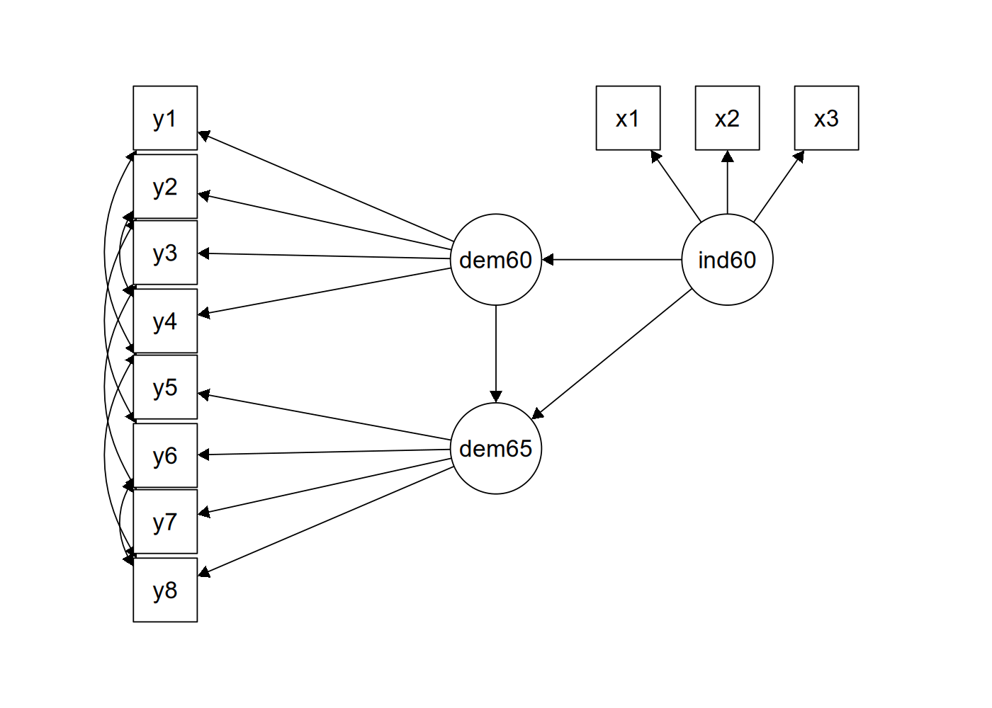
The figure below contains a graphical representation of the model that we want to fit.
The corresponding lavaan syntax for specifying this model is as follows:
model <- '
  # measurement model
    ind60 =~ x1 + x2 + x3
    dem60 =~ y1 + y2 + y3 + y4
    dem65 =~ y5 + y6 + y7 + y8
  # regressions
    dem60 ~ ind60
    dem65 ~ ind60 + dem60
  # residual correlations
    y1 ~~ y5
    y2 ~~ y4 + y6
    y3 ~~ y7
    y4 ~~ y8
    y6 ~~ y8
'
In this example, we use three different formula types: latent variable definitions (using the =~ operator), regression formulas (using the ~ operator), and (co)variance formulas (using the ~~ operator). The regression formulas are similar to ordinary formulas in R. The (co)variance formulas typically have the following form:
variable ~~ variableThe variables can be either observed or latent variables. If the two variable names are the same, the expression refers to the variance (or residual variance) of that variable. If the two variable names are different, the expression refers to the (residual) covariance among these two variables. The lavaan package automatically makes the distinction between variances and residual variances.
In our example, the expression y1 ~~ y5 allows the residual variances of the two observed variables to be correlated. This is sometimes done if it is believed that the two variables have something in common that is not captured by the latent variables. In this case, the two variables refer to identical scores, but measured in two different years (1960 and 1965, respectively). Note that the two expressions y2 ~~ y4 and y2 ~~ y6, can be combined into the expression y2 ~~ y4 + y6, because the variable on the left of the ~~ operator (y2) is the same. This is just a shorthand notation.
We enter the model syntax as follows:
model <- '
  # measurement model
    ind60 =~ x1 + x2 + x3
    dem60 =~ y1 + y2 + y3 + y4
    dem65 =~ y5 + y6 + y7 + y8
  # regressions
    dem60 ~ ind60
    dem65 ~ ind60 + dem60
  # residual correlations
    y1 ~~ y5
    y2 ~~ y4 + y6
    y3 ~~ y7
    y4 ~~ y8
    y6 ~~ y8
'
To fit the model and see the results we can type:
fit <- sem(model, data = PoliticalDemocracy)
summary(fit, standardized = TRUE)
lavaan 0.6-21 ended normally after 68 iterations
Estimator ML
Optimization method NLMINB
Number of model parameters 31
Number of observations 75
Model Test User Model:
Test statistic 38.125
Degrees of freedom 35
P-value (Chi-square) 0.329
Parameter Estimates:
Standard errors Standard
Information Expected
Information saturated (h1) model Structured
Latent Variables:
Estimate Std.Err z-value P(>|z|) Std.lv Std.all
ind60 =~
x1 1.000 0.670 0.920
x2 2.180 0.139 15.742 0.000 1.460 0.973
x3 1.819 0.152 11.967 0.000 1.218 0.872
dem60 =~
y1 1.000 2.223 0.850
y2 1.257 0.182 6.889 0.000 2.794 0.717
y3 1.058 0.151 6.987 0.000 2.351 0.722
y4 1.265 0.145 8.722 0.000 2.812 0.846
dem65 =~
y5 1.000 2.103 0.808
y6 1.186 0.169 7.024 0.000 2.493 0.746
y7 1.280 0.160 8.002 0.000 2.691 0.824
y8 1.266 0.158 8.007 0.000 2.662 0.828
Regressions:
Estimate Std.Err z-value P(>|z|) Std.lv Std.all
dem60 ~
ind60 1.483 0.399 3.715 0.000 0.447 0.447
dem65 ~
ind60 0.572 0.221 2.586 0.010 0.182 0.182
dem60 0.837 0.098 8.514 0.000 0.885 0.885
Covariances:
Estimate Std.Err z-value P(>|z|) Std.lv Std.all
.y1 ~~
.y5 0.624 0.358 1.741 0.082 0.624 0.296
.y2 ~~
.y4 1.313 0.702 1.871 0.061 1.313 0.273
.y6 2.153 0.734 2.934 0.003 2.153 0.356
.y3 ~~
.y7 0.795 0.608 1.308 0.191 0.795 0.191
.y4 ~~
.y8 0.348 0.442 0.787 0.431 0.348 0.109
.y6 ~~
.y8 1.356 0.568 2.386 0.017 1.356 0.338
Variances:
Estimate Std.Err z-value P(>|z|) Std.lv Std.all
.x1 0.082 0.019 4.184 0.000 0.082 0.154
.x2 0.120 0.070 1.718 0.086 0.120 0.053
.x3 0.467 0.090 5.177 0.000 0.467 0.239
.y1 1.891 0.444 4.256 0.000 1.891 0.277
.y2 7.373 1.374 5.366 0.000 7.373 0.486
.y3 5.067 0.952 5.324 0.000 5.067 0.478
.y4 3.148 0.739 4.261 0.000 3.148 0.285
.y5 2.351 0.480 4.895 0.000 2.351 0.347
.y6 4.954 0.914 5.419 0.000 4.954 0.443
.y7 3.431 0.713 4.814 0.000 3.431 0.322
.y8 3.254 0.695 4.685 0.000 3.254 0.315
ind60 0.448 0.087 5.173 0.000 1.000 1.000
.dem60 3.956 0.921 4.295 0.000 0.800 0.800
.dem65 0.172 0.215 0.803 0.422 0.039 0.039The function sem() is very similar to the function cfa(). In fact, the two functions are currently almost identical, but this may change in the future. In the summary() function, we omitted the fit.measures = TRUE argument. Therefore, you only get the basic chi-square test statistic. The argument standardized = TRUE augments the output with standardized parameter values. Two extra columns of standardized parameter values are printed. In the first column (labeled Std.lv), only the latent variables are standardized. In the second column (labeled Std.all), both latent and observed variables are standardized. The latter is often called the ‘completely standardized solution’.
The complete code to specify and fit this model is printed again below:
library(lavaan) # only needed once per session
model <- '
  # measurement model
    ind60 =~ x1 + x2 + x3
    dem60 =~ y1 + y2 + y3 + y4
    dem65 =~ y5 + y6 + y7 + y8
  # regressions
    dem60 ~ ind60
    dem65 ~ ind60 + dem60
  # residual correlations
    y1 ~~ y5
    y2 ~~ y4 + y6
    y3 ~~ y7
    y4 ~~ y8
    y6 ~~ y8
'
fit <- sem(model, data=PoliticalDemocracy)
summary(fit, standardized=TRUE)